09:33 Thwaites Researcher 2.3 cracked | |
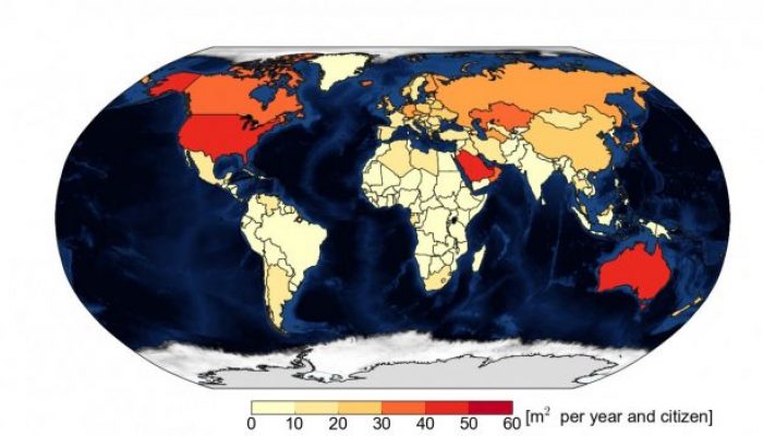
climate change Mean area of Arctic September sea ice lost by CO 2 emissions of each citizen for each country of the world in 2013. These results are based on the observed trend of 3 m² climate change
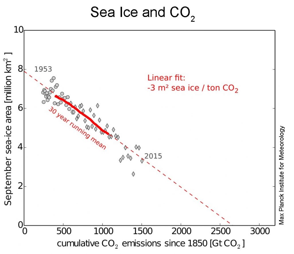
Mean area of Arctic September sea ice lost by CO2 emissions of each citizen for each country of the world in 2013. These results are based on the observed trend of 3 m² sea-ice area loss per tonne of CO2 emitted [Credit: adapted from Notz and Stroeve (2016), Fig.S1 ] Declining sea ice in the Arctic is definitely one of the most iconic consequences of climate change. In a study recently published in Science. Dirk Notz and Julienne Stroeve find a linear relationship between carbon dioxide (CO2 ) emissions and loss of Arctic sea-ice area in summer. Our image of this week is based on these results and shows the area of September Arctic sea ice lost per inhabitant due to CO2 emissions in 2013. What did we know about the Arctic sea ice before this study?Since the late 1970s, sea ice has been dramatically shrinking in the Arctic. losing 3.8% of its area per decade. Sea-ice area is at its minimum in September, at the end of the melting season. How exactly is sea-ice loss related to CO2 emissions ?Notz and Stroeve (2016) relate the Arctic sea-ice decline to cumulative CO2 emissions since 1850 (i.e. the total amount of CO 2 that has been emitted since 1850) for both observations and climate models. Cumulative CO2 emissions constitute a robust indicator of the recent man-made global warming (IPCC, 2014 ). The two quantities are clearly linearly related (see Figure 2). From 1953 to 2015, about 3.5 million km² of Arctic sea ice have been lost in September while 1200 gigatonnes (1 Gt = 10e 9 tonnes) of CO2 have been emitted to the atmosphere. This means that for each tonne of CO2 released into the atmosphere, the Arctic loses 3 m² of sea ice.
Fig 2: Monthly mean September Arctic sea-ice area against cumulative CO2 emissions since 1850 for the period 1953-2015. Grey circles and diamonds show the results from in-situ (1953-1978) and satellite (1979-2015) observations, respectively. The thick red line shows the 30-year running mean and the dotted red line represents the trend of 3 m² sea-ice area loss per tonne of CO2 emitted. [Credit: D. Notz, National Snow and Ice Data Center ] Starting from the relationship between cumulative CO2 emissions and sea-ice area, it is then easy to attribute to each country in the world their own contribution to sea-ice loss based on their CO2 emissions per capita. The countries that stand out in the map are thus the countries emitting the most in relation to their population. Could the Arctic be ice-free in the future?Edited by Clara Burgard and Sophie Berger Further reading
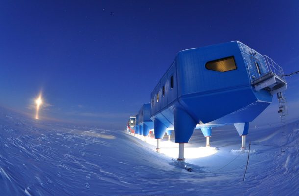
Halley VI research station. [Credit: British Antarctic Survey]. On theBrunt Ice Shelf, Antarctica, a never-observed-before migration has just begun. As the pale summer sun allows the slow ballet of the supply vessels to restart, men and machines alike must make the most of the short clement season. It is time. At last, the Halley VI research station is on the move! Halley, sixth of its nameDue to the inhospitable nature of Antarctica, there have been six successive Halley research stations:
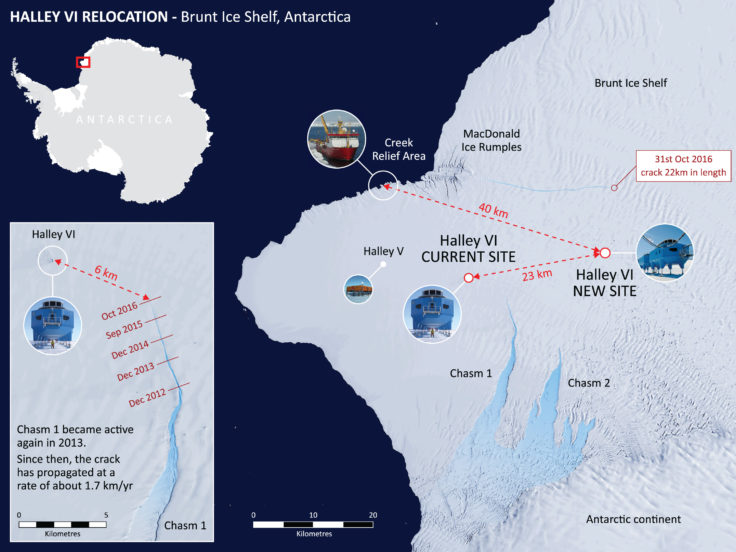
The relocation project, featuring the new October crack. Inset, timeline of the awakening of Chasm 1. The ice shelf flows approximately from right to left. [Credit: British Antarctic Survey ]. The awakening of the cracksThe project of moving Halley VI was announced a year ago. A very deep crack in the ice (“Chasm 1” in the map above) upstream of the station and dormant for 35 years, started growing again barely a year after the opening of Halley VI. The risk of losing the station if this part of the ice shelf broke off as an iceberg became obvious, and it was decided to move the station upstream &%238211; beyond the crack. Additionally, there is another problem, or rather another crack, which appeared last October. This one is located north of the station and runs across a route used to resupply Halley VI. This means that of the two locations where a supply ship would normally dock, one is no longer connected to the research station and hence rather useless. Not only is the station now encircled by deep cracks, now it also has only one resupply route remaining; to bring equipment, personnel and food and fuel supplies to the station &%238211; all of which are needed to successfully pull off the station relocation. Bringing Halley VI to its new location before the end of the short Antarctic summer season will be a challenge. We shall certainly keep you up-to-date with Halley news as well as with news about the rapid changes of the Brunt Ice Shelf (because we’re the Cryosphere blog after all!). In the meantime, you can feel like a polar explorer and enjoy this (virtual) visit of Halley VI . References and further readingEdited by Clara Burgard, Sophie Berger and Emma Smith
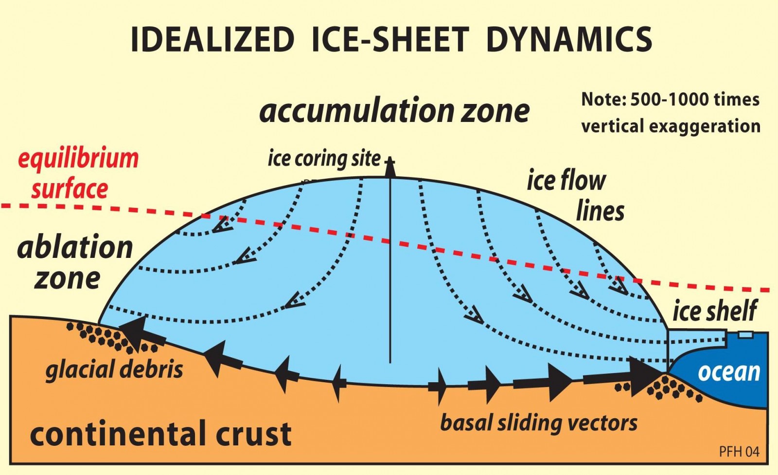
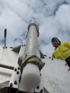
Ice sheets, archives of our past&%238230;We drill ice cores &%238211; of course!An ice core is a cylinder of ice that is retrieved from the ice sheet by drilling vertically downwards. The core is drilled in sections from the surface, deep into the ice sheet (Fig. 1) using a rotating drill. Each section of the core is processed at the drill site and often cut further into shorter sections of 55 cm for more practical transport and analysis in labs. A great deal of equipment is needed to achieve this and drilling is a slow and careful process often taking several field seasons to drill a deep core. An example of a drilling camp is shown in Fig. 2, housing scientists and engineers involved in drilling an ice core on the Fletcher Promontory, West Antarctica.
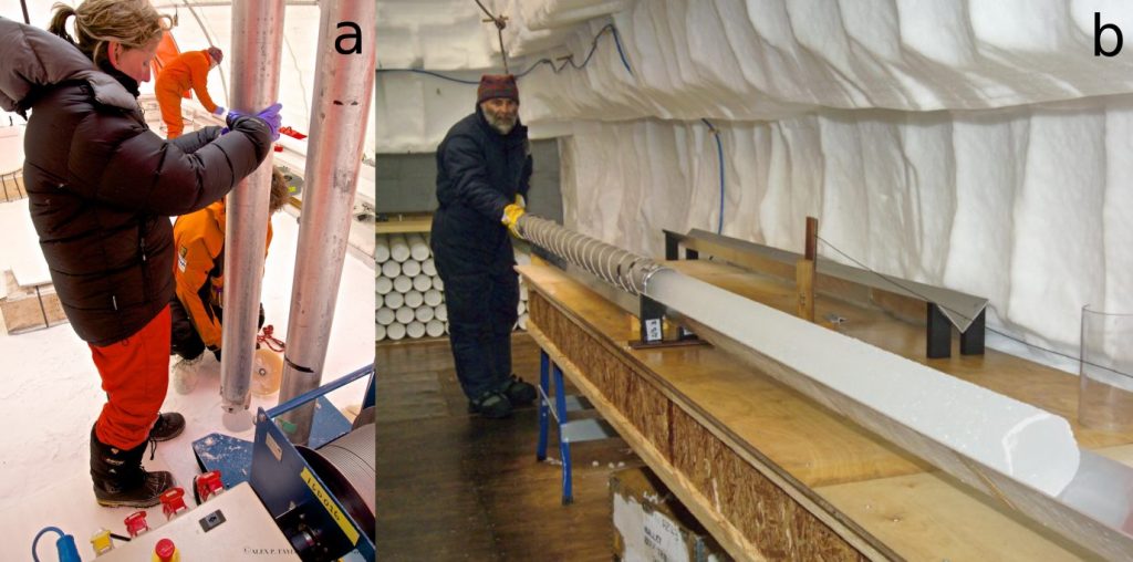
Figure 1: a) Ice core drill being lowered into the ice on Pine Island Glacier [Credit: Alex P. Taylor] b) Dr Rob Mulvaney processing the Berkner Island ice core, Weddell Sea, Antarctica [Credit: R. Mulvaney]
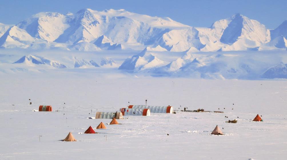
Figure 2: The layout of the Fletcher Promontory ice-drilling project, Weddell Sea, Antarctica. In the background the large Weatherhaven tent houses the drill rig, the central Weatherhaven tent is used for storage and equipment and a simple shower, the nearest Polarhaven tent is the mess tent, and the Polarhaven tent to the left houses the main generator. The pyramid tents in the foreground are the sleeping tents, and the two to the right are used for toilet facilities [Credit: Mulvaney et al. 2014 ] Where to drill an ice core for the best record?
Figure 3: Ice flow within the ice sheet showing the zero flow at the ice divide &%238211; the ideal site for an ice core [Credit: Snowball Earth ] If your aim is to find the oldest ice on Earth, East Antarctica is a good place to start looking What does an ice core actually record?Once an ice core has been drilled and cut into sections, some of the sections are analysed and others are preserved. This is particularly important as some of the analysis is destructive (e.g. melting of the ice to extract water and gas). Therefore an archive of the ice core itself is needed. So, what information can we obtain from analysing the core and how is it done? Annual layers, past snowfall and past temperatures!Reconstructing the past surface temperature and snowfall is incredibly useful for understanding climate processes and changes through time in order to assess any present-day local and regional changes in climate. We can do this by:
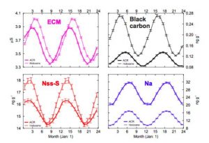
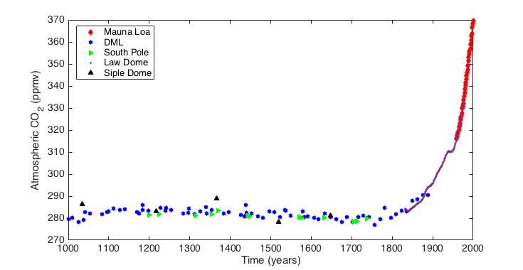
Figure 4: Seasonal deposition of four chemical species in the WAIS Divide ice core. Pink: electrical conductivity measurements; Black: Black Carbon; Red: non-sea salt Sulphur; Blue: Sodium. Each panel, shows the averaged annual record for 2 different periods: the Antarctic Cold Reversal (ACR, 13-14,000 years ago – bold line) and the Holocene, (10-11,000 years ago – thin line) the [Credit: Fig. 2, Sigl et al. 2016 ] The deposition of a number of chemical elements increases during the summer season and decreases during the winter.When these elements are measured in the ice core they can be depicted as an almost-sinusoidal record, indicating the historical seasons. High-resolution ice-core profiles can be dated by counting these annual layers, and have been done so across Greenland and at the West Antarctic Ice Sheet (WAIS) Divide ice core site. Fig. 4 shows two annual signals over 24 months for four different chemicals that are deposited in ice cores (Sigl et al. 2016 ). The peak in seasonal deposition is shown twice for each chemical, at different times in history, but the seasonality of these species remains strong throughout time. Atmospheric gasIce-core measurements of atmospheric gases correlate well with direct measurements taken from the atmosphere dating back to 1950. As a result of this, ice-core scientists can assume that the atmospheric gas concentrations measured in ice cores reflects the atmospheric conditions at the time the gas was entrapped in the ice core. Hence, ice cores tell us that carbon dioxide concentrations have been relatively stable for the last millennia until around 1800 AD but since then a rise of almost 40% has been measured in both ice cores and direct atmospheric measurements (Fig. 5).
Carbon dioxide concentrations have been relatively stable for the last millennia until around 1800 AD but since then a rise of almost 40% has been measured
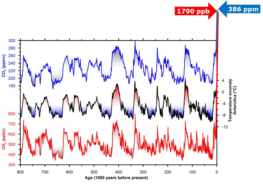
Figure 6: Variations of temperature (from present day mean temperature, black), atmospheric carbon dioxide (in part per million by volume &%238212; blue) and methane (in part per billion per volume red) over the past 800,000 years, from the EPICA Dome C ice core in Antarctica. Modern value (of 2009) of carbon dioxide and methane are indicated by arrows. [Credit. Centre for Ice and Climate. University of Copenhagen. Re-used with permission ] Other climate proxiesChemistry preserved in the ice also offers a proxy (=a means) to reconstruct other seasonally-deposited tracers:
Current knowledge from ice-core recordsAs we have seen, ice core are important because they put the current climate variations into the context of a long-term climate history. Additionally, polar ice cores can allow us to looks at variations between the northern and southern hemisphere. Ice cores also extend back much, much further in time than terrestrial weather stations or satellite records:
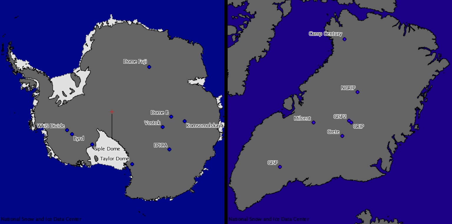
Figure 7: Deep ice core locations in Greenland and Antarctica [Credit and more details: NSIDC ] The current past climate record tells us about glacial and inter-glacial periods (Fig. 6) but also allows us to look at finer detail &%238211; i.e. the variability within these periods, which were previously assumed stable. For example, ice cores have led to the discovery of Dansgaard-Oeschger events; which are are rapid climate fluctuation events, characterised by rapid warming followed by gradual cooling to return to glacial conditions, 25 of these events have happened during the last glacial period. Records from the Northern and Southern hemisphere also allow us to link these small and large scale changes in climate in the two hemispheres. For example, ice cores analysed from both poles show a ‘call and response’ signal between Dansgaard-Oeschger events in the Northern Hemisphere and events in the Antarctic climate record. The southern hemisphere cooled during the warm phases of Dansgaard-Oeschger events in the northern hemisphere ( Buizert et al. 2015 ). and vice versa during northern hemispheric cooling (see our previous blog post on the subject). There are already over a dozen ice cores taken from Greenland and Antarctica (Fig. 7), offering a clear and detailed history of the climate during the Late Quaternary period (Fig. 6), going back up to 800,000 years (Quaternary = last 2.6 million years). As we mentioned earlier the timing of glacial and inter-galcial cycles in this 800,000 year old record is dominated by the orbital cycle of the Earth (96,000-year periodicity). However, marine records show that frequency of glacial-interglacial cycles was different before this time (Lisiecki and Raymo, 2005 ). It is in order to better understand these changes that the quest for the oldest was formed &%238211; beginning last month the mission aims to drill an ice core of ice older than 800,000 years to gain detailed information about the climate even further back in time. Edited by Emma Smith and Sophie Berger
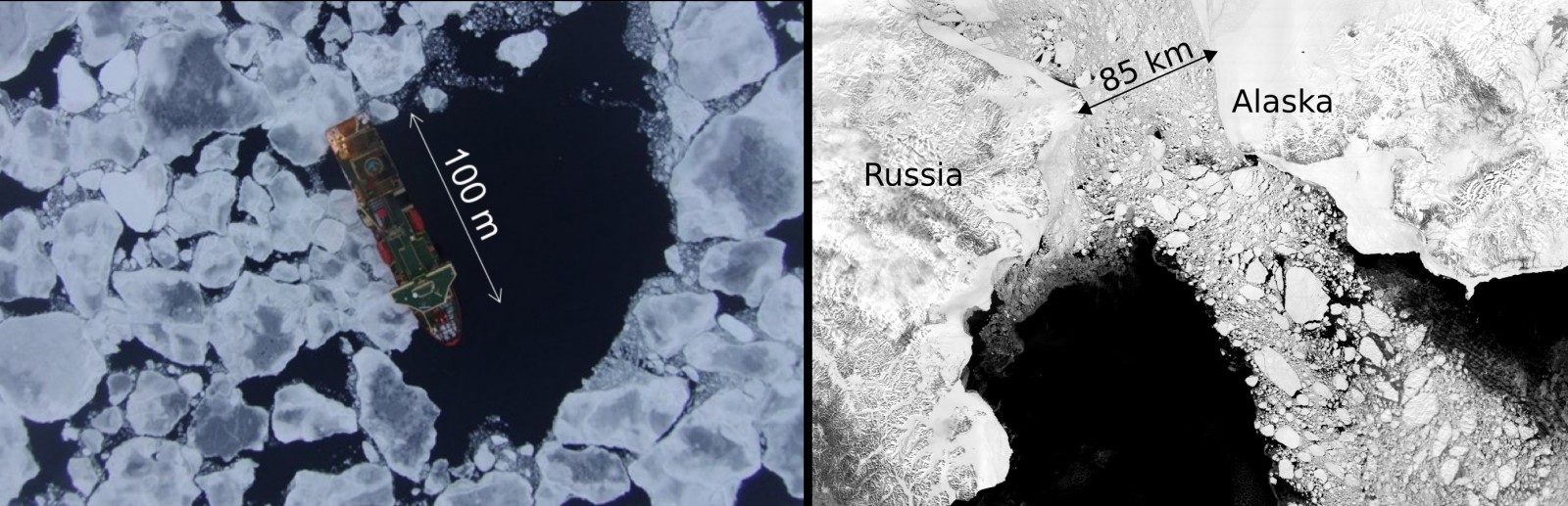
The polar regions are covered by a thin sheet of sea ice &%238211; frozen water that forms out of the same ocean water it floats on. Often, portrayals of Earth’s sea ice cover show it as a great, white, sheet. Looking more closely, however reveals the sea ice cover to be a varied and jumbled collection of floating pieces of ice, known as floes. The distribution and size of these floes is vitally important for understanding how the sea ice will interact with its environment in the future. [Read More]
There is million-year old ice somewhere deep under the surface of the Antarctic ice sheet! [Credit: Brice Van Liefferinge] This is it! The new European horizon 2020 project on Oldest Ice has been launched and the teams are already heading out to the field, but what does “Old Ice” really mean? Where can we find it and why should we even care? This is what we (Marie, Olivier and Brice) will try to explain somewhat. Why do we care about old ice, ice cores and past climate?
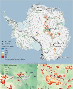
Figure 1: Drilling an ice core [Credit: Brice Van Liefferinge] Unravelling past climate and how it responded to changes in environmental conditions (e.g. radiative forcing) is crucial for our understanding of the current climate and for predicting how climate will likely change in the future. Ice cores contain unique and quantitative information on the past climate (e.g. atmospheric gas concentration). The caveat is that at the moment, we can “only” go back up to 800,000 years at EPICA Dome C ice core (Parrenin et al, 2007 ). The new European project &%238216;Oldest ice&%238217; was set up for this very objective: crack the Mid-Pleistocene Transition climate.It brings together engineers, experimentalists and modellers from 14 Universities around the world. In this post, we will focus on the first mission of the project: locating areas with million year old ice in Antarctica. The next steps will be to: develop the drilling technology, improve our geophysical knowledge of the identified site, and finally, reach the “holy grail”: recover ice from the very base of the ice sheet with a target age of 1.5 Million years. The whole project is anticipated to last 10 years! The new European project &%238216;Oldest ice&%238217; was set up for this very objective: crack the Mid-Pleistocene Transition climate The first mission: “Where to find million year old ice?”Oldest Ice (ice more than 1 mio. years old) can only be recovered in Antarctica, but where exactly? This question has to be answered in a two-step approach: On a large scale, we must first narrow down places in Antarctica where Oldest Ice might be found. To do that, we rely on models. Then, we can focus our analysis on those regions by gathering field data in the form of airborne radar surveys. Further ground-based work is currently taking place. On a larger scale, Oldest Ice in Antarctica requires:Thick ice and cold bed. We need thick ice to reconstruct past climate variations with sufficient temporal resolution (e.g. is there enough ice to measure air bubbles or other climate markers). However, the thicker the ice, the higher the basal temperature. If the bottom of the ice is too warm, the ice at the base will start to melt, potentially destroying the Oldest Ice of the ice sheet.
Figure 2. Potential locations of cold bed (basal temperatures 2000 m), slow motion (horizontal flow speeds <2m/yr) The colour bar represents the basal temperature. The two insets focus on Dome C and Dome F, two areas highly likely to store million year old ice. [Credit: Brice Van Lieffering, updated from Van Liefferinge, B. and Pattyn. 2013] While boundary conditions such as ice thickness and accumulation rates are relatively well constrained, the major uncertainty remains in determining thermal conditions at the ice base. The thermal conditions depend on the geothermal heat flow (the flux of &%238220;energy&%238221; provided by the Earth which conducts heat into the crust) underneath the ice sheet. But to measure the geothermal heat flow, you need to reach the bed. Give it a go: Try to find million year old ice yourself using this Matlab© tool: http://homepages.ulb.ac.be/ On finer scales: we need deep radiostratigraphy and age modellingRadar profiles
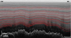
Figure 3. Radargram from the new Oldest Ice A radar survey (Young et al. in review) with isochrones interpreted in red [Credit: Marie Cavitte] This allows to date entire sub-regions. However, the very bottom of the ice column is often difficult to interpret: radar isochrones cannot always be continuously followed from the ice core. Radargrams are powerful tools to observe the internal structure of the ice The newly acquired Oldest Ice A radar survey (Young et al. in review ) over the Dome C region (see figure 2 for location) gives very rich stratigraphic information and the proximity of the EPICA Dome C ice core has allowed the dating of the isochrones. The ice sheet in this area could only be dated to 360,000 years (Cavitte et al. 2016 ) and not further back in time because deeper isochrones are tricky to tie to the ice core, and other times, there is no clear signal (deep scattering ice, visible near the bedrock, at the bottom of Figure 3). As such, we need an age model to try to describe the age-depth relation below the deepest dated isochrones. Modelling the ice
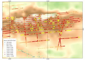
Figure 4. More precise analysis of the Dome C Oldest Ice target, with the lines representing the Oldest Ice A airborne survey collected in winter 2015/16 (Young et al. in review). The colours represent the modelled age of the ice 60 meters above the bedrock, in thousands of years. We can see that this whole region has a lot of potential for recovering million year old ice. [Credit: Olivier Passalacqua] The age of the ice primarily depends on its vertical velocity, so we can use a simple 1D model to describe the motion of the ice in the vertical direction. We run the model for an ensemble of vertical velocity profiles and basal melt rates, and consider the distribution of the basal ages (i.e. model ages) given by the profiles that reproduce the observations the best (i.e. isochrones ages). We need an age model to try to describe the age-depth relation below the deepest dated isochrones After running the model, it appears that many areas of the Oldest Ice A survey region host very old ice (see red and yellow dots on figure 4 which represent ages > 1 million years). A high enough bottom age gradient, provided by the dated isochrones, is required to ensure sufficiently old ice as a drilling target. Following initial calculations, it will probably be a better choice to drill on the flank of the bedrock relief than on its top. So in the end, where do we find the oldest ice?To find out more about Beyond EPICA and keep track of progress visit the project website and follow @OldestIce on twitter! Brice Van Liefferinge is a PhD student and a teaching assistant at the Laboratoire de Glaciology, Université libre de Bruxelles, Belgium. His research focuses on the basal conditions of the Antarctic ice sheet. H e tweets as @bvlieffe . Marie Cavitte is a PhD student at the Institute for Geophysics at the University of Texas at Austin, Texas. Her research focuses on understanding radar internal stratigraphy and using it as a means to constrain the temporal stability of the East Antarctic Ice Sheet interior. Olivier Passalacqua is a PhD student at the Laboratoire de G laciologie et Géophysique de l&%238217;Environnement, Grenoble, France. Members of the consortiumInstitute for Geophysics, University of Texas at Austin (UTIG, US) Australian Antarctic Division (AAD, Australia)
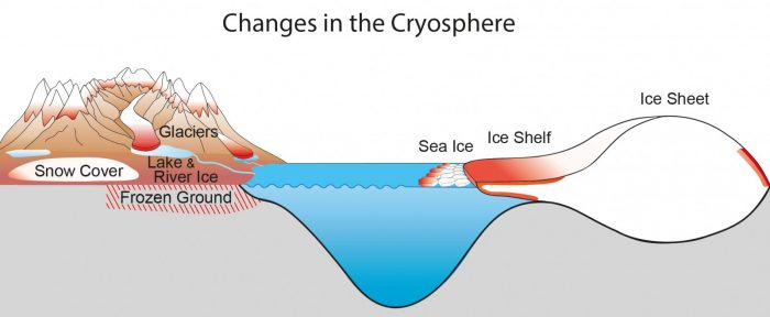
Schematic summary of the dominant observed variations in the cryosphere. [Credit: fig 4.25 from IPCC (2013) ]. In this new political context, we must not forget about the scientific evidence of climate change! Our figure of the week, today summarises how climate change affects the cryosphere, as exposed in the latest assessment report of the Intergovernmental Panel on Climate Change (IPCC, 2013, chapter 4) Observed changes in the cryosphereGlaciers (excluding Greenland and Antarctica)Sea Ice in the Arctic
Ice Shelves and ice tongues
Ice Sheets
Permafrost/Frozen Ground
Snow cover
Lake and river ice
Further readingHow much can President Trump impact climate change?Thwaites Researcher 2.3 cracked Free DownloadThwaites Researcher 2.3 cracked FREE DOWNLOAD | |
|
| |
 David Docquier is a post-doctoral researcher at the Earth and Life Institute of Université catholique de Louvain (UCL) in Belgium. He works on the development of processed-based sea-ice metrics in order to improve the evaluation of global climate models (GCMs). His study is embedded within the EU Horizon 2020 PRIMAVERA project, which aims at developing a new generation of high-resolution GCMs to better represent the climate.